path: root/index.md

---
pagetitle: yummers
lang: en
---
# histogram-preserving tri-planar projection
31 March 2026

I've been messing around with Burley's "On Histogram-Preserving Blending for
Randomized Texture Tiling" ([link](https://jcgt.org/published/0008/04/02/)) for
a couple days. The core idea is to pre-process images into a "Gaussianized"
form where the histogram of the image's colors follows a Gaussian distribution.
Once in Gaussian form, there is a closed-form way to blend multiple samples with
barycentric weights such that the Gaussian's variance is preserved (Equation 2
in the paper). Finally, you can run the blended colors through a lookup table
(LUT) to get a result in the original image's color space. The results are
outstanding. (These ideas build on those laid out by Heitz and
Neyret in an earlier paper. I will reference Heitz a few times.)

![Heitz style tiling material comparison. Left = naive tiling, right = tiling
using Heitz's per-pixel histogram-preserving blending operator.](./images/2026_03_31/Screenshot from 2026-03-31 19-59-45.jpg)

It was love at first sight - you can use this to seamlessly tile large areas
with textures that themselves don't even need to be seamless. However, the
method uses 4 taps per pixel (3 overlapping hexagons per pixel, plus 1 3D
lookup table tap).

I've been thinking about terrains for a week or two, since I need to make a
large-scale environment for a project. I really like the idea of using
tri-planar projection for grass, stone etc., but I've never been satisfied with
the quality I get from it. It always creates this awful loss of contrast
between layers and creates weird ghosting artifacts.

Wait a minute, isn't that kind of what Heitz's technique addresses?

It turns out that yeah, you can use the exact same machinery described by Heitz
and Burley to perform histogram-preserving tri-planar projection.
You just use standard tri-planar projection to get barycentric
coordinates instead of playing with a UV-space triangle grid. Results are shown
below.

![Left to right: control; naive tri-planar projection; histogram-preserving
tri-planar projection.](./images/2026_03_31/results.jpg)

I also noticed that the gamma term described in Burley's Equation 5 can
significantly reduce contrast. At low values, where ghosting is more visible,
contrast is better preserved; at high values, it's more diminished.


![Left to right: gamma=0.5, 1, 2, 4, 8](./images/2026_03_31/results_gamma.jpg)

Perhaps blending in YCbCr would ameliorate the loss in contrast, but I haven't
tried that yet.

The astute reader might find that just increasing contrast after the blend
would produce a similar result, and I'm inclined to agree. The only possible
advantage that this method has is that it doesn't demand fine-tuning.

# using linux as a desktop os in 2026
9 Feb 2026

About a month ago, my PC's boot drive died. I had been running Windows 11 with
moderate dissatisfaction for a few months, so I decided to switch over to
Linux as my primary OS. These are some notes on that process. My
motivation is to give an accurate portrayal of what to expect out of the
switching process and the day-to-day operation.

TLDR: The Linux desktop is *way* better in 2026 than it was in 2016. Native app
support is far more common, and Proton is really good. If dual booting was not
still necessary for VR, I would wholeheartedly recommend it.

## Dual boot setup

I knew immediately that I'd be dual booting. My memory told me that some apps
just would not work well, and the virtualization tax is high, so I'd want a
native Windows install. So I made my first mistake: I installed Linux, *then*
Windows. The opposite order is far more streamlined. So I just overwrote my
install with Win11. I left half my drive as unallocated space for the Linux
install.

After rebooting normally to make sure Windows was really working, it was time
to install Linux. My new install would not let me get into BIOS - my keyboard
inputs did not work. There are one-time flags you can set via shell (PowerShell
and BASH) to do various boot-related tasks without keyboard input. To get into
BIOS:

* PowerShell: `shutdown /r /fw /t 0`
* bash: `sudo systemctl reboot --firmware-setup`

My keyboard did work once in the BIOS, so I was then able to enter my Linux
bootable USB. I had some trouble getting the bootable USB to work. I had to
install the media via Rufus's `dd` mode instead of the default.

I installed my distro as normal in the unallocated space, then rebooted. GRUB
showed up, showing my Linux install as default and the Windows boot manager
below. Somewhat unsurprisingly, my keyboard didn't work in GRUB. I heard that
disabling fast boot and
[xhci](https://en.wikipedia.org/wiki/Extensible_Host_Controller_Interface)
handoff in the BIOS can help, but this only temporarily helped before the issue
resurfaced and then resolved itself. My current config has fast boot off and
xhci handoff off.

My solution to the pre-BIOS/GRUB keyboard issue is just to use shell commands
to reboot. To get from Windows to Linux, I just reboot as normal since Linux
has prio by default in my install. To go from Linux to Windows, I installed
`efibootmgr`, ran it to get the numeric ID of the Windows boot manager (0000),
then crafted this one liner:

* bash: `sudo efibootmgr --bootnext 0000 && reboot`

I use ctrl+R to find it every time I need to reboot.

> Sidebar: this method does not play nicely with Windows updates. Since
> Windows needs to reboot 19 times to do anything, and each reboot takes you
> into Linux, you'll be stuck booting back into Windows manually. Next time
> Windows demands an update, I'll probably just unplug my PC from the wall.

## Linux setup

I'm using the Ubuntu 2024 LTS as my distro. My first point of confusion getting
started was the apparent surfeit of package managers: apt (the standard),
snap (canonical's thing), and flatpak (some semi popular community thing).
snap and flatpak are sandboxed by default, which is really just a massive
fucking pain in the ass for GUI apps. So I use apt wherever possible, and raw
.deb files for the rest.

### Audio

Audio's a little scuffed, but seems like we've mostly gotten on the pulse audio
train (thank God).

For whatever reason, my motherboard's audio output sets itself to 39% volume. I
have to use `alsamixer` to increase this to 100%.

I used `pavucontrol` to disable irrelevant speakers and mics s.a. monitor speakers.

### Firefox

Firefox comes pre-installed on Ubuntu. Firefox is slowly going the way of
Windows, but [Just The Browser](https://justthebrowser.com/) has some easy one
liners to de-shittify it. Waterfox is also interesting, but I haven't tried it
yet.

### Discord

I used the raw .deb to install Discord. It will ask you to manually update
every few days. I wrote this shell script to speed that up:

```bash
#!/usr/bin/env bash
# updisc: update discord

set -o errexit
set -o xtrace

cd $HOME/Downloads
wget --content-disposition "https://discord.com/api/download/stable?platform=linux&format=deb"
latest=$(ls -v | grep discord | tail -n1)
sudo dpkg -i "$latest"
```

### Spotify

The snap works fine for this. Installed it through the App Center (Canonical's
app store).

(Preachy note: Spotify kind of sucks. Avoid using their auto generated
playlists. Spotify has something called the Perfect Fit Program which
commissions and pushes music to listeners based on non-public preference data.
Artists involved in this program are not well compensated. Read about it in Liz
Pelly's
[expose](https://harpers.org/archive/2025/01/the-ghosts-in-the-machine-liz-pelly-spotify-musicians/).)

### Steam

I use the raw .deb to install Steam. I tried the flatpak at first, but the
sandboxing doesn't play nicely with proton. Steam will keep itself up to date
so the raw .deb is fine.

### Games

I had some issues with graphics drivers in certain games and had to roll back
my driver from 590 to 570. You can list your driver with `nvidia-smi`, and
install some other version (e.g. 570) with `sudo apt install
nvidia-driver-570`. It will ask for a password - this only has to be entered
once after reboot, after which the driver will be trusted forever.

If your game uses Easy Anti Cheat and Proton, you'll need to install the Proton
EasyAntiCheat runtime. It should be listed in your library by default.

Proton has a heavy FPS hit vs. Windows native (like 30%), but I'm not a
competitive gamer and my computer is very over-built, so I don't care.

### Blender

I downloaded the LTS .tar.xz from the website and put it in my bin directory. I
think it's probably smarter to use Steam for this. Do *not* use the snap
version - it won't let you install addons from the web.

If you use an NDOF input device like a spacemouse, install
[spacenavd](https://github.com/FreeSpacenav/spacenavd) via apt. You might have
to relaunch blender.

Otherwise, pretty much identical experience.

### Unity

Superficially, Unity basically just works. Install the hub using the official
Unity3D [documentation](https://docs.unity3d.com/hub/manual/InstallHub.html#install-hub-linux).

My problems with Unity so far are:

* Slow shader compile times.
* Unity uses OpenGL by default on Linux, and Vulkan is very crashy in my
  experience.
  * OpenGL uses a different depth buffer format than DX11/DX12, making it hard
    to develop for that platform on the OpenGL version.
* GPU profiler doesn't work out of the box, showing 1 ms for every frame.
* Weird permissions issues if you just mount a project created in Windows. Had
  to copy it over.
* Have to delete Library/ if the project was created/used on Windows.
  (Shouldn't be a big deal. Just slows down first time startup.)
* Slow scrolling performance in Inspector pane
* Dragging sliders in game mode is not smooth, like it is in Windows

You can use ALCOM/vrc-get to create VRChat projects. Get it [from
github](https://github.com/vrc-get/vrc-get).

### Adobe

I've already been on Krita (and GIMP before that), which natively supports
Linux. No problems there.

Substance painter is a massive issue. Adobe claims to have a native Ubuntu build,
and even sell it through Steam. However, it simply did not launch on my
system. It was missing half a dozen shared object files (.so), and after
manually fixing that it still fails to launch.

Thankfully the fuckwits at Adobe couldn't be bothered to strip their binary:

```
$ file ./Adobe\ Substance\ 3D\ Painter
./Adobe Substance 3D Painter: ELF 64-bit LSB pie executable, x86-64, version 1 (GNU/Linux), dynamically linked, interpreter /lib64/ld-linux-x86-64.so.2, for GNU/Linux 3.2.0, BuildID[sha1]=cf49a257fa3bcf0f40d860a8a45a67c873571421, with debug_info, not stripped
$ $ du -h ./Adobe\ Substance\ 3D\ Painter
305M    ./Adobe Substance 3D Painter
```

So the next time I have a free afternoon I'll be looking through that.

I did try ArmorPaint, but it is very clearly still quite early in development.
I do not think that it's a viable alternative to Substance Painter yet. (For
example: you cannot drag and drop in textures, nor can you import more than one
at a time. Functional, sure, but barely.) To its credit: unlike Substance
Painter, it actually launches.

## Pleasant surprises

Linux is way, way more polished than I remember it. Back in college I was
fucking around with Arch (and didn't know what I was doing) so I was expecting
a far more painful setup process. Instead it was very seamless. Audio works
well. There are very few weird audio/graphical bugs. NVIDIA drivers are easy to
install. Gaming basically just works - I have yet to encounter a game which I
can't play (I've only tried maybe a dozen).

The amount of native app support is really heartwarming. Skipping over the big
apps like Firefox and Steam, here are some smaller apps I was surprised to see
native support for:

* OBS (video recording/streaming tool)
* Factorio (indie game)
* r2modman (mod manager)
* Chatterino (twitch chat app)
* PureRef (artist reference app)
* Lorien (infinite canvas drawing app)

## Complaints

Canonical uses the "yes/maybe later" pattern which degrades the notion of
consent. Nearly every large firm does it now since Google about-faced a couple
years ago, but it is still a grave degradation of user rights that shouldn't be
glossed over.

SteamVR does not work for me. My knuckles did not have an internally
consistent coordinate system, preventing me from completing room
calibration.
I was never able to figure this out. This~~, along with Unity's crashy behavior
on Vulkan,~~* is what's keeping me from just deleting Windows.

\* I've actually been able to use the OpenGL build to do graphical programming
  without issue for a few weeks now. So, not an issue.

## Conclusions

The Linux desktop is really good. You should give it a try.

# hemi-octahedral impostors
14 Jan 2026

*Note: this blog post is only like half way complete. I may or may not circle
back to it. The stuff on octahedral mappings is all finished, but the
impostor application below is not.*

Ryan Brucks published [an
article](https://shaderbits.com/blog/octahedral-impostors) describing
"octahedral impostors" in 2018. The basic idea is to to take photos of some
subject at octahedral lattice points, record them to an atlas, then reconstruct
those photos in a particle.

![Octahedral lattice points around some object.](./images/2026_01_14/Screenshot from 2026-01-14
13-35-40.png)

## But why octahedrons?

The octahedral mapping is simply one way to convert between a flat coordinate
system and a spherical coordinate system. It is notable because it does not use
any trig functions, making it suitable for use in realtime graphics.

This is what an octahedron looks like:

![Unit octahedron.](./images/2026_01_14/Screenshot from 2026-01-14
13-54-05.png)

It is a polyhedron with 8 triangular faces and 6 vertices. The equator is a
square.

Let's work out how we'd convert this octahedron to a plane.
First, we project the upper hemisphere onto the xz plane:

![Octahedron with upper hemisphere projected onto xz
plane.](./images/2026_01_14/Screenshot from 2026-01-14 13-50-27.png)

Next, we effectively need to "rotate" the triangles in the lower half around
those diagonal edges. We can cheat by first *reflecting* the bottom vertex of each
triangle about its diagonal edge:

![Octahedron with reflected lower hemisphere.](./images/2026_01_14/Screenshot from 2026-01-14 13-58-18.png)

Finally, we can just project those points in the lower hemisphere onto the xz
plane:

![Fully unwrapped octahedron.](./images/2026_01_14/Screenshot from 2026-01-14 13-59-24.png)

Viewed head on, we can see a very beautifully symmetric unwrapping:

![Unwrapped octahedron, head on.](./images/2026_01_14/Screenshot from 2026-01-14 14-00-16.png)

Note that we never actually did any rotations, so there no trig! Here's the
same procedure in code:

```c
// Convert unit octahedron to a [-1,1] x [-1,1] patch on xz plane.
float3 octahedron_to_plane(float3 p) {
  if (p.y >= 0) {
    // Project upper hemisphere onto xz plane.
    p.y = 0;
    return p;
  }
  // First, reflect the lower hemisphere's points about their diagonal.
  p.x = sign(p.x) * (1 - abs(p.x));
  p.z = sign(p.z) * (1 - abs(p.z));
  // Then project onto the xz plane.
  p.y = 0;
  return p;
}
```

We can generalize this procedure to unwrap *any* spherical object by just
switching norms:

```c
// Convert unit sphere to a [-1,1] x [-1,1] patch on xz plane.
float3 octahedron_to_plane(float3 p) {
  // Switch from L2 to L1 norm. This basically bends a sphere to an octahedron.
  float l1_norm = abs(p.x) + abs(p.y) + abs(p.z);
  p /= l1_norm;
  // Then unwrap.
  if (p.y < 0) {
    p.x = sign(p.x) * (1 - abs(p.x));
    p.z = sign(p.z) * (1 - abs(p.z));
  }
  p.y = 0;
  return p;
}
```

Here's a quick demo showing what that norm conversion does to a unit sphere:

![Converting a sphere to an octahedron via norm conversion.](./images/2026_01_14/hemi_octahedral_04.mp4)

Going from plane to octahedron is just the same thing backwards:

```c
// Convert a [-1,1] x [-1,1] patch on xz plane to a unit sphere.
float3 plane_to_octahedron(float3 p) {
  float l1_norm = abs(p.x) + abs(p.z);
  if (l1_norm > 1) {
    // Reflect lower hemisphere's point about their diagonal.
    p.x = sign(p.x) * (1 - abs(p.x));
    p.z = sign(p.z) * (1 - abs(p.z));
  }
  p.y = 1 - l1_norm;
  return normalize(p);
}
```

If you'd like more discussion on this topic, I recommend the spherical geometry section in [the PBR book](https://www.pbr-book.org/4ed/Geometry_and_Transformations/Spherical_Geometry#x3-OctahedralEncoding).)

## The hemi octahedron

We might only want to map the upper hemisphere to a plane. In that case, we can
first note that in the standard octahedral mapping, the inner diamond of the
[-1,1] x [-1,1] square gets mapped to the upper hemisphere. So all we have to
do is first remap our input to that diamond via a scale and 45 degree rotation, map it,
then rotate it back. The code is still very simple:

```c
// Convert unit sphere to a [-1,1] x [-1,1] patch on xz plane.
float3 hemi_octahedron_to_plane(float3 p) {
  // Rotate 45° and scale to fit square into diamond
  float x_rot = (p.x + p.z) * 0.5;
  float z_rot = (p.z - p.x) * 0.5;
  p.x = x_rot;
  p.z = z_rot;

  float l1_norm = abs(p.x) + abs(p.y) + abs(p.z);
  p /= l1_norm;
  if (p.y < 0) {
    p.x = sign(p.x) * (1 - abs(p.x));
    p.z = sign(p.z) * (1 - abs(p.z));
  }
  p.y = 0;

  // Rotate back.
  x_rot = p.x - p.z;
  z_rot = p.x + p.z;
  p.x = x_rot;
  p.z = z_rot;

  return p;
}
```

Here is that transform, visualized:

![Converting a hemi octahedron to a plane.](./images/2026_01_14/hemi_octahedral_05.mp4)

If we didn't do that scale and rotate, this is what it would look like:

![Converting a hemi octahedron to a plane.](./images/2026_01_14/hemi_octahedral_06.mp4)

I will leave the plane -> hemi-octahedron code as an exercise for the reader.

## Impostor v1

With this mapping, we can write some code to spawn cameras at the lattice
points of an octahedral-mapped hemisphere, pointing in at some target object,
and generate an atlas of images taken at different angles:

![Camera lattice points.](./images/2026_01_14/Screenshot\ from\ 2026-01-14\ 15-13-03.png)

![Generated atlas.](./images/2026_01_14/Impostor_atlas.png)

We can then write a naive particle shader which computes its nearest lattice
point and simply renders that image.

We can simply compute the direction from the camera to the particle's center,
map that to 2D using the hemi-octahedral mapping, then find the nearest lattice
point by rounding. We can also rotate the particle to the same orientation that
the photo was taken at to avoid any weird behavior when viewed top down.

That looks like this:

![Grid snapped impostor.](./images/2026_01_14/hemi_octahedral_07.mp4)

The popping is pretty awful! Can we do better?

## Impostor v2

Brucks describes a "virtual frame projection" method. I'll let him explain it:

> Looking back to the 'virtual grid mesh' above, we can see that for any triangle on the grid, it has 3 vertices. So if we want to blend smoothly across this grid, we need to be able to identify the 3 nearest frames. And remember how using a sprite caused messed up projection of just one frame? Well it turns out the same thing happens when you try to reuse the projection from one frame for another! This is a pain. So you actually have to render a virtual frame projection for the other 2 frames to simulate their geometry. While using the mesh UVs for one projection and 'solving' the other two does work, it falls apart for lower (~8x8) frame counts because the angular difference can be so great between cards that you see the card start to clip at grazing angles (not shown in any videos yet). As a compromise, the shader does not use ANY UVs right now. It solves all 3 frames using virtual frame projection in the vertex shader and then uses a traditional sprite vertex shader. The only downside is at close distances you occasionally see some minor clipping on the edge but it is much more acceptable this way.

Lost? Me too! I found this paragraph extremely confusing - it's what motivated
me to write this article.

As near as I can tell, what he's describing is that you retrieve
the nearest 3 lattice points and do a barycentric interpolation. He's also
trying to clarify that you can't just use the uvs from one lattice point to
sample another - you have to calculate each lattice point's uvs separately.
(I suppose that that level of optimization-first thinking is required when
you're building for Fortnite!)

You then render the blended color that on a standard facing quad primitive.

To start, I calculate the ray from the camera to the origin of the particle's
coordinate system. I use that position for my barycentric interpolation.

That looks like this:

![Barycentric interpolated impostor.](./images/2026_01_14/hemi_octahedral_08.mp4)

Huh. Looks a lot worse than his demo. What are we doing wrong?

Could it just be our choice of mesh that makes our results look bad? Here's Suzanne:

![Sus-anne.](./images/2026_01_14/hemi_octahedral_09.mp4)

Maybe it looks a little better?

The mesh that Brucks shows off in his blog post has radial symmetry and smooth
normals, which might be responsible.

You can also see some artifacts appearing in open space. This was caused by a
couple things:

1. The other mesh was toggled on when I generated my impostor atlas.
2. The bounding sphere around my mesh had very little padding.
3. The particle can rotate, and if you don't clip the parts outside the
   impostor's bounding sphere, you can wind up rendering them.

3 is crucial - with that correction in place, you can pack your atlas
pretty tightly. Here's Suzanne with that correction in place:

![Sus-anne 2.](./images/2026_01_14/hemi_octahedral_10.mp4)

Here's the atlas. Pretty tight packing - could probably be optimized a little
further though:

![Sus-anne atlas.](./images/2026_01_14/suzanne_atlas.png)

## Impostor v3

After stepping away for a bath, the issue occurred to me.

I was calculating the lattice point based on the direction from the camera to
the particle center. With barycentric interpolation in place, we would be
better off using a per-pixel ray intersection with the impostor's bounding
sphere. Concretely: we want to sample the lattice points whose cameras have a
direction most closely matching the standard view direction. This is found by
simply going from the particle's bounding sphere origin to the surface along
`-viewDir`, projecting that to 2d, then rounding to lattice points as normal.

This seems to help a bit, but it's not night and day. I didn't capture any
videos here, but the next gen uses this tech.

## Impostor v4

So far we've only been rendering pre-lit images of our subject on an unlit
particle. Can we do better? What if we captured the albedo, normal, metallic
gloss, and position, then lit it with a standard surface shader?

The results look a bit better - specular is much better approximated now:

![First true PBR impostor.](./images/2026_01_14/hemi_octahedral_11.mp4)

## Impostor v5

I continued to spin my wheels for a couple days. I re-read Brucks' article
several more times, and came to a couple conclusions:

1. He is using the camera-origin ray, not a per pixel view direction ray.
2. He is doing some form of parallax occlusion mapping to limit popping.

I found his description on
[this video](https://www.youtube.com/watch?v=6rsXe6kKTC4) useful:

> This version blends the three nearest frames using a single parallax offset (similar to a bump offset). This is the version of impostors used in FNBR on PC and Consoles. It was used on mobile originally but switched back to single frame at last minute since we were compositing them into HLODs and thus rendering lots of them.

That single parallax offset is explained by this image:

![Parallax offset
calculation.](https://storage.googleapis.com/wzukusers/user-22455410/images/5aadebd9593beeF0JN4n/UVParallax.JPG)

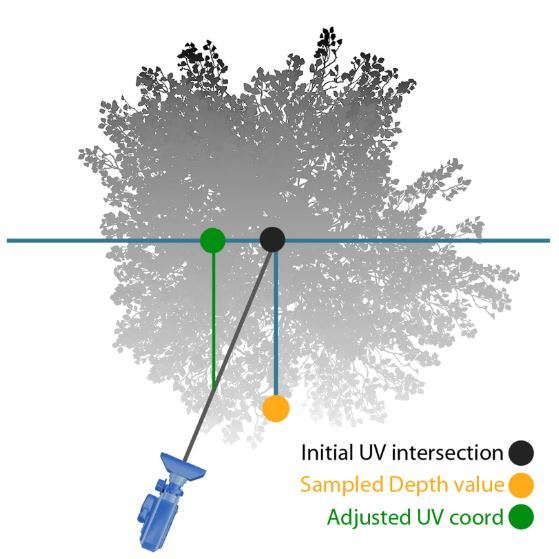
My buggy implementation looks promising - see how the eyes are much sharper
now?

![Impostor with 1 depth aware parallax correction.](./images/2026_01_14/hemi_octahedral_11.mp4)

It is still very, very poppy, unlike Brucks' demo. I must be doing something
wrong.

*Note: I stepped away from this project and don't plan to revisit it soon. If I
do, I'll post updates in a followup and link to it from here.*

# 6 wave dispersion relations with derivatives
21 Sep 2025

Tessendorf's 2005 paper
"[Simulating Ocean Water](https://people.computing.clemson.edu/~jtessen/reports/papers_files/coursenotes2004.pdf)"
describes three basic dispersion relations:

1. The deep water dispersion relation:

    $$
    \omega^2 = gk
    $$

    where $\omega$ is the wave's temporal frequency in $\text{rad}/s$, $g$ is gravity
    in $m/s^2$, and $k$ is the spatial frequency in $m/s$.

2. The shallow water dispersion relation:

    $$
    \omega^2 = gk \tanh kh
    $$

    where $h$ is the water mean depth in $m$.

3. The deep water relation with viscosity correction:

    $$
    \omega^2 = gk (1 + k^2 L^2)
    $$

    where $L$ is the scale in $m$ at which the viscosity term operates. At 0,
    it has no effect.

Horvath's 2015 paper
"[Empirical directional wave spectra for computer graphics](https://dl.acm.org/doi/10.1145/2791261.2791267)"
formulates the viscosity term in terms of different physical units, and applies
it to the shallow water dispersion relation:

$$
\omega^2 = (gk + \frac{\sigma}{\rho} k^3) \tanh kh
$$

where $\sigma$ is the surface tension in $N/m$, and $\rho$ is the water density
in $kg/m^3$.

It is useful to have derivatives of the dispersion relation. Horvath's paper
describes how we can calculate the spectrum term $S(k_x, k_y)$ from
$S(\omega, \theta)$ and the derivative of the dispersion relation
$\frac{\partial \omega}{\partial k}$:

$$
S(k_x, k_y) = S(\omega, \theta) \frac{\partial \omega}{\partial k} / k
$$

So, with that motivation, we would like the derivatives of our dispersion
relations. You should autodifferentiate if that's an option. If not, here are
derivations of each derivative:


1. Deep water:

    $$
    \begin{align*}
    \omega^2 &= gk \\
    \omega &= (gk)^\frac{1}{2} \\
    \frac{\partial \omega}{\partial k} &= \frac{1}{2} (gk)^{-\frac{1}{2}} g \\
    &= \frac{g}{2\sqrt{gk}} \\
    &= \frac{1}{2} \sqrt{\frac{g}{k}}
    \end{align*}
    $$

    Wolfram [here](https://www.wolframalpha.com/input?i=d%2Fdk+%28%28gk%29%5E%281%2F2%29%29).

2. Shallow water:

    First we will need $\frac{\partial}{\partial k} \tanh kh$:

    $$
    \begin{align*}
    \frac{\partial}{\partial k} \tanh kh
    &= \frac{\partial}{\partial k} [\frac{e^{kh} - e^{-kh}}{e^{kh}+e^{-kh}}] \\
    &= \frac{\partial}{\partial k} [(e^{kh} - e^{-kh})(e^{kh}+e^{-kh})^{-1}] \\
    &= (he^{kh}-he^{-kh})(e^{kh}+e^{-kh})^{-1} +
            (e^{kh}-e^{-kh})[-(e^{kh}+e^{-kh})^{-2}(he^{kh}-he^{-kh})] \\
    &= h(1-[\frac{e^{kh}-e^{-kh}}{e^{kh}+e^{-kh}}]^2 \\
    &= h(1-\tanh^2 kh)
    \end{align*}
    $$

    With that identity, let's proceed:

    $$
    \begin{align*}
    \omega^2 &= gk \tanh kh \\
    \omega &= (gk \tanh kh)^{\frac{1}{2}} \\
    \frac{\partial \omega}{\partial k} &= \frac{1}{2} [gk \tanh kh]^{-\frac{1}{2}} [g \tanh (kh) + gkh(1 - \tanh ^2 kh] \\
    &= \frac{g(\tanh kh + kh(1 - \tanh ^2 kh))}{2 \sqrt{gk \tanh kh}} \\
    &= \frac{g \tanh kh + gkh (1 - \tanh^2 kh)}{2 \sqrt{gk \tanh kh}} \\
    &= \frac{1}{2} [\sqrt{g \tanh kh} + \frac {gkh(1 - \tanh^2 kh)}{\sqrt{gk \tanh kh}}] \\
    &= \frac {g \tanh kh + gkh(1 - \tanh^2 kh)}{2\sqrt{gk \tanh kh}} \\
    &= \frac {g (\tanh kh + kh \operatorname{sech}^2 kh)}{2\sqrt{gk \tanh kh}}
    \end{align*}
    $$

    Wolfram [here](https://www.wolframalpha.com/input?i=d%2Fdk+%5Bsqrt%28gk+tanh+%28kh%29%29%5D).
    (Recall that $\operatorname{sech}^2 x = 1 - \tanh^2 x$.)

3. Viscous deep water (Tessendorf version):

    $$
    \begin{align*}
    \omega^2 &= gk [1 + k^2 L^2] \\
    \omega &= (gk [1 + k^2 L^2])^{\frac{1}{2}} \\
    \frac{\partial \omega}{\partial k} &= \frac{1}{2}(gk [1 + k^2 L^2])^{-\frac{1}{2}} [g+3gk^2 L^2] \\
    &= \frac{g+3gk^2L^2}{2\sqrt{gk[1+k^2L^2]}}
    \end{align*}
    $$

    Wolfram [here](https://www.wolframalpha.com/input?i=d%2Fdk+%5B%28gk+%281+%2B+%28k%5E2%29+%28L%5E2%29%29%29+%5E+%281%2F2%29%5D).

4. Viscous deep water (Horvath version):

    $$
    \begin{align*}
    \omega^2 &= gk + \frac{\sigma}{\rho}k^3 \\
    \omega &= (gk + \frac{\sigma}{\rho}k^3)^{\frac{1}{2}} \\
    \frac{\partial \omega}{\partial k} &=
            \frac{1}{2}(gk + \frac{\sigma}{\rho}k^3)^{-\frac{1}{2}} [g+3\frac{\sigma}{\rho}k^2] \\
    &= \frac{g + 3 \frac{\sigma}{\rho}k^2}{2 \sqrt{gk+\frac{\sigma}{\rho}k^3}}
    \end{align*}
    $$

    Wolfram [here](https://www.wolframalpha.com/input?i=d%2Fdk+%5B%28gk%2Bs%28k%5E3%29%2Fp%29%5E%281%2F2%29%5D).

5. Viscous shallow water (Tessendorf version):

    FYI - use the Horvath version instead. This relation sucks.

    We'll want $\frac{\partial}{\partial k} \sqrt{\tanh kh}$:

    $$
    \begin{align*}
    \frac{\partial}{\partial k} \sqrt{\tanh kh}
    &= \frac{\partial}{\partial k} (\tanh kh)^{\frac{1}{2}} \\
    &= \frac{1}{2} (\tanh kh)^{-\frac{1}{2}} \frac{\partial}{\partial k} \tanh kh \\
    &= \frac{1}{2} (\tanh kh)^{-\frac{1}{2}} h(1 - \tanh^2 kh) \\
    &= h \frac{1 - \tanh^2 kh}{2 \sqrt{\tanh kh}} \\
    &= h \frac{\operatorname{sech}^2 kh}{2 \sqrt{\tanh kh}}
    \end{align*}
    $$

    Now we can proceed:

    $$
    \begin{align*}
    \omega^2 &= gk (1 + k^2 L^2) \tanh kh \\
    \omega &= (gk (1 + k^2 L^2) \tanh kh)^{\frac{1}{2}} \\
    \frac{\partial \omega}{\partial k}
    &= (\frac{\partial}{\partial k} [gk (1 + k^2 L^2)]) \tanh kh +
        [gk (1 + k^2 L^2)] \frac{\partial}{\partial k} \tanh kh \\
    &= \frac{g (3 + k^2 L^2)}{2 \sqrt{k} \sqrt{g (1 + k^2 L^2)}} \dots \\
    &= \frac{1}{2} \sqrt{\frac{g(3+k^2 L^2)}{k}} \sqrt{\tanh kh} +
            \sqrt{gk (1+k^2 L^2)} [\frac{h (1 - \tanh^2 kh)}{2 \sqrt{\tanh kh}}]
    \end{align*}
    $$

    We can apply some transformations to get a common denominator and agree
    with Wolfram:

    $$
    \begin{align*}
    \frac{\partial \omega}{\partial k}
    &= \frac{g (3 + k^2 L^2)}{2 \sqrt{gk(1+k^2 L^2)}} \sqrt{\tanh kh} + \dots \\
    &= \frac{g (3 + k^2 L^2) \tanh kh}{2 \sqrt{gk(1+k^2 L^2) \tanh kh}} + \dots \\
    &= \dots + \sqrt{gk (1+k^2 L^2)} [\frac{h (1 - \tanh^2 kh)}{2 \sqrt{\tanh kh}}] \\
    &= \dots + \frac{gk(1+k^2 L^2)}{\sqrt{gk(1+k^2 L^2)}} [\frac{h (1 - \tanh^2 kh)}{2 \sqrt{\tanh kh}}] \\
    &= \dots + \frac{gk(1+k^2 L^2) h (1 - \tanh^2 kh)}{2 \sqrt{gk(1+k^2 L^2) \tanh kh}} \\
    &= \dots + \frac{ghk(1+k^2 L^2)(1-\tanh^2 kh)}{2 \sqrt{gk(1+k^2 L^2) \tanh kh}} \\
    &= \frac{g(3+k^2L^2) \tanh kh + ghk(1+k^2 L^2)(1-\tanh^2 kh)}{2 \sqrt{gk(1+k^2 L^2) \tanh kh}} \\
    &= \frac{g(3+k^2L^2) \tanh kh + ghk(1+k^2 L^2)(\operatorname{sech}^2 kh)}{2 \sqrt{gk(1+k^2 L^2) \tanh kh}}
    \end{align*}
    $$

    Wolfram [here](https://www.wolframalpha.com/input?i=d%2Fdk+%5Bsqrt%28gk+%281+%2B+%28k%5E2%29%28L%5E2%29%29+tanh+%28kh%29%29%5D).

6. Viscous shallow water (Horvath version):

    $$
    \begin{align*}
    \omega^2 &= (gk + \frac{\sigma}{\rho}k^3) \tanh kh \\
    \omega &= ((gk + \frac{\sigma}{\rho}k^3) \tanh kh)^{\frac{1}{2}} \\
    \frac{\partial \omega}{\partial k}
    &= [\frac{\partial}{\partial k}(gk + \frac{\sigma}{\rho}k^3)] \tanh^{\frac{1}{2}} kh +
        (gk + \frac{\sigma}{\rho}k^3)^{\frac{1}{2}} \frac{\partial}{\partial k} \tanh^{\frac{1}{2}} kh \\
    &= [\frac{1}{2}(gk+\frac{\sigma}{\rho}k^3)^{-\frac{1}{2}}(g+3\frac{\sigma}{\rho}k^2)] \tanh^{\frac{1}{2}} kh +
        (gk + \frac{\sigma}{\rho}k^3)^{\frac{1}{2}}h\frac{1-\tanh^2 kh}{2 \sqrt{\tanh kh}}
    \end{align*}
    $$

    Let's try to corral this into a form closer to what Wolfram gives us:

    $$
    \begin{align*}
    \frac{\partial \omega}{\partial k}
    &= [\frac{1}{2}(gk+\frac{\sigma}{\rho}k^3)^{-\frac{1}{2}}(g+3\frac{\sigma}{\rho}k^2)] \sqrt{\tanh{kh}} +
        (gk + \frac{\sigma}{\rho}k^3)^{\frac{1}{2}}h\frac{1-\tanh^2 kh}{2 \sqrt{\tanh kh}} \\
    &= \frac{g+3\frac{\sigma}{\rho}k^2}{2\sqrt{gk+\frac{\sigma}{\rho}k^3}} \sqrt{\tanh{kh}} + \dots \\
    &= \frac{(g+3\frac{\sigma}{\rho}k^2) \tanh{kh}}{2\sqrt{(gk+\frac{\sigma}{\rho}k^3)\tanh{kh}}} + \dots \\
    &= \dots + (gk + \frac{\sigma}{\rho}k^3)^{\frac{1}{2}}h\frac{1-\tanh^2 kh}{2 \sqrt{\tanh kh}} \\
    &= \dots + (gk + \frac{\sigma}{\rho}k^3)h\frac{1-\tanh^2 kh}{2 \sqrt{(gk + \frac{\sigma}{\rho}k^3) \tanh kh}} \\
    &= \dots + \frac{h (gk+\frac{\sigma}{\rho}k^3) (1 - \tanh^2 kh)}{2 \sqrt{(gk+\frac{\sigma}{\rho}k^3)\tanh kh}} \\
    &= \frac{(g+3\frac{\sigma}{\rho}k^2) \tanh{kh} + h (gk+\frac{\sigma}{\rho}k^3) (1 - \tanh^2 kh)}{2 \sqrt{(gk+\frac{\sigma}{\rho}k^3)\tanh kh}} \\
    &= \frac{(g+3\frac{\sigma}{\rho}k^2) \tanh{kh} + h (gk+\frac{\sigma}{\rho}k^3) \operatorname{sech}^2{kh}}{2 \sqrt{(gk+\frac{\sigma}{\rho}k^3)\tanh kh}}
    \end{align*}
    $$


    Wolfram [here](https://www.wolframalpha.com/input?i=d%2Fdk+%5B%28%28gk%2Bs%28k%5E3%29%2Fp%29tanh%28kh%29%29%5E%281%2F2%29%5D).
    Divide numerator and denominator by $\rho$ (or p in wolfram) to make them
    match.

# meow meow meow meow
10 Sep 2025

meow meow meow meow meow meow meow meow'meow meow meow meow meow. meow
meow meow meow.

## meow meow

* meow meow meow 3 meow meow 65 meow meow meow.
  * 3% meow meow meow meow meow meow meow 3 meow.
  * meow meow meow meow meow meow meow meow meow 65 meow.
* meow meow meow meow meow meow 1-10 meow meow meow.
  * meow meow meow meow meow'meow meow meow meow meow meow-meow meow meow meow meow
    meow meow meow meow. meow, meow meow meow meow meow meow meow.
* meow meow > 3 meow meow meow meow meow meow meow meow.
* meow meow meow meow meow 10 meow/meow^2 meow'meow meow. meow'meow meow
  meow meow meow meow meow.

## meow, meow: meow meow meow meow meow (2007)

[meow meow meow.](meow://meow.meow.meow.meow/meow/meow/meow/meow43-48-meow2007.meow)

meow

* meow 1993, meow meow meow meow meow meow meow meow meow meow.
* meow 1997, meow meow meow meow meow 560 meow meow. 76% meow meow meow
  meow meow. (meow'meow meow meow meow meow 1, meow 38)
* meow 2012, meow meow meow meow meow meow meow 30 meow meow.
* meow meow meow, meow meow meow 2, meow meow 2 meow meow
  meow meow meow meow.
* meow 1 meow 4,000 meow meow meow meow meow meow (meow).
  * meow meow meow meow 5% meow meow meow meow.

meow

* meow meow meow meow meow meow.
* meow meow meow meow meow meow meow meow meow meow.
* 25% meow meow meow meow meow meow meow meow 20meow meow 30meow.
* 25% meow meow meow meow meow meow meow. meow meow meow meow
  meow meow.

meow meow meow

* 79%: meow meow meow
* 10%: meow meow
* 6%: meow meow
* 5%: meow meow

meow meow

* meow meow meow meow meow meow (meow)
* meow meow meow meow meow meow meow meow meow
* meow meow meow 1362 meow meow meow meow
  * (meow: 1 meow/meow^2 meow meow meow 1 *meow*)
* meow meow meow meow 5 meow meow meow, 5 meow meow meow.
* meow meow meow 0-12 meow. meow meow meow.
* meow meow, meow meow meow meow meow meow meow meow meow 3 meow 65
  meow.
* 49% meow meow meow meow meow meow meow 50 meow, meow meow meow meow
  meow meow meow meow meow meow meow meow meow (meow meow meow
  meow).
* meow meow meow meow meow meow meow meow meow.
* 67% meow meow meow meow meow meow meow meow meow meow.
* meow

meow meow

* meow meow meow meow meow
* meow meow meow meow meow meow meow meow meow meow meow meow meow
* meow meow meow meow meow meow
* meow meow meow meow 1-10 meow meow meow
  * meow: meow 120 meow meow, meow meow meow meow meow meow 1200 meow meow 2400
    meow *meow*. meow!
* meow meow meow meow meow meow 10-20 meow meow meow meow.
* meow meow meow meow meow meow meow meow.

meow meow

* meow meow > 3 meow meow meow meow meow meow meow 25% meow meow meow meow
  meow.
  * meow meow meow meow meow meow meow meow meow 10 meow meow meow.
* meow meow meow meow meow meow 3 meow meow meow meow *meow*.

## meow, meow: meow meow meow meow meow meow meow
meow (2002)

[meow meow meow.](meow://meow.meow/2001-150.meow)

meow

* meow 1 meow 6000 meow meow meow meow meow
* meow meow meow meow meow 7 meow 20 meow meow
* (meow meow meow meow meow meow meow)
* meow meow meow meow meow meow meow meow meow meow meow meow meow meow meow
  meow meow meow meow meow meow, meow meow meow meow.

meow

* meow meow meow, meow meow-meow meow, meow meow meow meow meow
  meow meow
* meow meow meow meow meow meow meow meow meow meow meow meow meow
  meow meow meow meow meow meow 1 meow 50 meow. meow meow meow
  meow meow meow (meow meow meow meow meow - 0% = meow meow, 100% =
  meow meow meow meow) meow meow meow 50% (meow meow).
* meow meow meow. meow meow meow meow meow meow meow meow meow
  meow meow meow 10 meow/meow^2 meow 200 meow/meow^2. meow 10meow/meow^2, meow meow meow
  meow; meow 200 meow/meow^2, meow meow. "... meow meow meow meow meow meow
  meow meow meow meow meow meow meow meow meow meow meow."
* meow meow 5 meow/meow^2 meow meow meow meow meow meow meow meow.
  meow meow 20 meow/meow^2 meow meow meow meow meow meow meow 100 meow/meow^2.
  * meow: meow meow = meow meow meow.
* meow meow meow meow meow meow meow meow meow meow meow,
  meow 8.8% meow meow meow meow meow ~55% meow meow meow meow.

# rasterized ray marching at scale
11 Jun 2025

I've long had the dream of creating high resolution chains on characters with
raymarching. The problem is that Unity's object transform is based on the
character's hip bone, so making raymarched geometry "stick" to characters
is impossible.

The idea I've been toying with for a long time is to raymarch inside a
rasterized box. If you store information in that box's verts, you could do a
raymarch inside a wholly self contained coordinate system.
I've pulled this off, but not in a way which is useful for characters (yet).


![One draw call, many raymarched objects.](./images/2025_06_11/fake_origins_31.png){width=80%}

TLDR:

* Create a Blender plugin to bake the location and orientation of submeshes.
  Plugin available
  [here](https://github.com/yum-food/2ner/blob/master/Scripts/BakeVertexData.py).
* Create a Unity script to visualize the baked data. Script available
  [here](https://github.com/yum-food/2ner/blob/master/Scripts/Editor/DecodeVertexData.cs).
* Provide HLSL code showing how to use the baked data.

## Main ideas and HLSL

The core idea is to make it possible for each fragment of a material to learn
an origin point's location and orientation. If you can recover an origin point
and a rotation, then you can raymarch inside that coordinate system, then
translate back to object coordinates at the end.

For each submesh\* in a mesh, I bake an origin point and an orientation.

\* A submesh is just a set of vertices connected by edges. A mesh might contain
many unconnected submeshes. For example, in blender, you can combine two
objects with ctrl+J. I call those two combined but unconnected things
*submeshes*.

The orientation of the submesh is derived from the face normals. I sort the
faces in the submesh by their area. The largest area face is used as the first
basis vector of our rotated coordinate system. Then I get the next face which
is sufficiently orthogonal to the first basis vector (absolute value of dot
product is > some epsilon). I orthogonalize those two basis vectors with
[graham-schmidt](https://en.wikipedia.org/wiki/Gram%E2%80%93Schmidt_process),
then generate the third with a cross product. I ensure right-handedness by
checking that the determinant is positive, then [convert to a
quaternion](https://en.wikipedia.org/wiki/Rotation_matrix#Conversion_from_rotation_matrix_to_axis%E2%80%93angle).
I then store that quaternion in 2 UV channels.

The rotation quaternion is recovered on the GPU as follows:

```c
float4 GetRotation(v2f i, float2 uv_channels) {
  float4 quat;
  quat.xy = get_uv_by_channel(i, uv_channels.x);
  quat.zw = get_uv_by_channel(i, uv_channels.y);
  return quat;
}
...
RayMarcherOutput MyRayMarcher(v2f i) {
...
  float2 uv_channels = float2(1, 2);
  float4 quat = GetRotation(i, uv_channels);
  float4 iquat = float4(-quat.xyz, quat.w);
}
```

It's worth lingering here for a second. Each submesh is conceptualized as a
rotated bounding box. We just deduced an orthonormal basis for that rotated
coordinate system. That means that the artist can rotate their bounding boxes
however they want in Blender, and the plugin will automatically work out how to
orient things. You can arbitrarily move and rotate your bounding boxes and it
Just Works.

The origin point is simply the average of all the vertex locations. I encode it
as a vector from each vertex to that location, and stuff it into vertex colors.
Since vertex colors can only encode numbers in the range [0, 1], I use the
alpha channel to scale the length of each vertex.

I made two non obvious decisions in the way I bake the vertex offsets:

1. The offsets are encoded in terms of the rotated coordinate system. This saves
   one quaternion rotation in the shader.

2. The offsets are scaled according to the L-infinity norm (Manhattan distance)
   rather than the standard L2 norm (Euclidian distance). This lets the artist
   think in terms of the bounding box dimensions rather than the square root of
   the sum of squares of the box's dimensions. Like if your box is 1x0.6x0.2,
   then you can just raymarch a primitive with those dimensions and your
   simulation Just Works.

The origin point is recovered on the GPU as follows:

```c
float3 GetFragToOrigin(v2f i) {
  return (i.color * 2.0f - 1.0f) / i.color.a;
}
RayMarcherOutput MyRayMarcher(v2f i) {
...
  float3 frag_to_origin = GetFragToOrigin(i);
}
```

With those pieces in place, the raymarcher is pretty standard, but some care
has to be taken when getting into and out of the coordinate system. Here's a
complete example in HLSL:

```c
RayMarcherOutput MyRayMarcher(v2f i) {
  float3 obj_space_camera_pos = mul(unity_WorldToObject,
      float4(_WorldSpaceCameraPos, 1.0));
  float3 frag_to_origin = GetFragToOrigin(i);

  float2 uv_channels = float2(1, 2);
  float4 quat = GetRotation(i, uv_channels);
  float4 iquat = float4(-quat.xyz, quat.w);

  // ro is already expressed in terms of rotated basis vectors, so we
  // don't have to rotate it again.
  float3 ro = -frag_to_origin;
  float3 rd = normalize(i.objPos - obj_space_camera_pos);
  rd = rotate_vector(rd, iquat);

  float d;
  float d_acc = 0;
  const float epsilon = 1e-3f;
  const float max_d = 1;

  [loop]
  for (uint ii; ii < CUSTOM30_MAX_STEPS; ++ii) {
    float3 p = ro + rd * d_acc;
    d = map(p);
    d_acc += d;
    if (d < epsilon) break;
    if (d_acc > max_d) break;
  }
  clip(epsilon - d);

  float3 localHit = ro + rd * d_acc;
  float3 objHit = rotate_vector(localHit, quat);
  float3 objCenterOffset = rotate_vector(frag_to_origin, quat);

  RayMarcherOutput o;
  o.objPos = objHit + (i.objPos + objCenterOffset);
  float4 clipPos = UnityObjectToClipPos(o.objPos);
  o.depth = clipPos.z / clipPos.w;

  // Calculate normal in rotated space using standard raymarcher
  // gradient technique
  float3 sdfNormal = calc_normal(localHit);
  float3 objNormal = rotate_vector(sdfNormal, quat);
  o.normal = UnityObjectToWorldNormal(objNormal);

  return o;
}
```

## Scalability and limitations

1. This technique is extremely scalable. I have a world with 16,000 bounding boxes
that runs at ~800 microseconds/frame without volumetrics.

2. You can have overlapping raymarched geometry without paying the usual 8x
slowdown of [domain
repetition](https://iquilezles.org/articles/sdfrepetition/).

![Overlapping geometry.](./images/2025_06_11/fake_origins_demo.mp4){width=80%}

You still pay the price of overdraw, and unlike domain repetition, there's no
built-in compute budgeting. I.e. with domain repetition you'd hit your
iteration cap and stop. With this you won't.

3. The workflow is artist friendly. You can move, scale, and rotate your
geometry freely. Re-bake once you're done and everything just works.

4. Shearing works, but doesn't permit re-baking.

![Test setup, no shearing](./images/2025_06_11/fake_origins_32.png){width=80%}

![Shear in Blender but don't
re-bake.](./images/2025_06_11/fake_origins_33.png){width=80%}

![Shear in Blender and
re-bake](./images/2025_06_11/fake_origins_34.png){width=80%}

![Shear in Unity.](./images/2025_06_11/fake_origins_35.png){width=80%}

## Blender and Unity tooling

I've written a Blender plugin to permit myself to bake the vectors and
quaternions as described above.

![Blender overview.](./images/2025_06_11/fake_origins_36.png){width=80%}

The plugin supports baking vectors and quaternions on extremely large meshes
primarily through caching. If your mesh contains many submeshes that are
simply translated in space, then baking should take less than a second. If
those submeshes are scaled, skewed, or rotated, then they won't cache and
baking will take longer.

The baker lets you rotate the baked quaternion around the basis vectors. I had
to fuck with this a fair bit, and eventually found that 180 degrees worked. Try
going through every combo of 90 degrees (64 total) if you run into trouble. Use
[quick exporter](https://github.com/Wildergames/blender-quick-exporter) to
speed up the process. You can visualize the vectors with my Unity script, which
is described below.

![Baker options.](./images/2025_06_11/fake_origins_38.png){width=80%}

It also supports a bunch of other workflows, mostly designed for the voxel
world creation workflow:

1. Select all linked submeshes. This just does ctrl+L for each submesh with at
least one vert, edge, or face selected. Blender's built in ctrl+L seems to be
inconsistent in its behavior.

2. Select linked across boundaries. This basically does ctrl+L, but lets the
meshes be disconnected at as long as they have a vert that's within some
epsilon of a selected vert. That epsilon is configurable. It's scalable
up to thousands of submeshes.

3. Deduplicate submeshes. This just looks for submeshes where all their verts
are close to others. The closeness parameter (epsilon) is configurable. It
works via spatial hashing so it's extremely scalable.

4. Merge by distance per submesh. This just iterates over all submeshes and
does a merge by distance on each. When working with large collections of
submeshes, it's easy to accidentally duplicate a face/edge/vert along the way,
and these duplications can stack up. This lets you recover.

5. Pack UV island by submesh Z. This lets you pack UV islands for large
collections of submeshes and sort them by their Blender z axis height. Buggy as
shit rn, sorry!

This is less relevant, but I wanted some way to instance axis-aligned geometry
along a curve and sort each instance's UVs by Z height. These nodes do that.
Put them on a curve and select your instance. Then use the "Pack UV island by
submesh Z" plugin tool to actually pack them.

![Instance axis-aligned geometry and sort
UVs.](./images/2025_06_11/fake_origins_37.png){width=80%}

Finally, I have a Unity script which lets you visualize the raw baked vectors,
and the "corrected" baked vectors, i.e. those rotated with the baked
quaternion. Simply attach "Decode vertex vectors" to your gameobject. The light
blue vectors are raw vectors, and the orange ones are the corrected ones. The
orange ones should converge at the center of each submesh.
(It's okay if they overshoot/undershoot, you
can correct for that in your SDF.)

![Visualize baked data in
Unity.](./images/2025_06_11/fake_origins_39.png){width=80%}

# how much CO2 do American cars produce?
23 May 2025

TLDR: About $1.520 \cdot 10^{12}$ kg/year. This increases the CO$_2$ in the
atmosphere by about $0.048$% per year.

Let's gather some facts:

* The average American (16 or older) drives about 13,476 miles per year
  ([US DoT](https://www.fhwa.dot.gov/ohim/onh00/bar8.htm)).
* There are 265,653,749 Americans aged 16 or older
  ([US 2020 Census](https://www2.census.gov/programs-surveys/popest/tables/2020-2023/national/asrh/nc-est2023-agesex.xlsx)).
* Finished motor gasoline releases about 18.73 pounds of CO$_2$ per gallon
  ([US Energy Information Administration](https://www.eia.gov/environment/emissions/co2_vol_mass.php)).
* New light duty vehicles (those weighing 10,000 pounds or less) get about 26.0
  miles per gallon (mpg) as of 2024
  ([US DoE](https://www.energy.gov/eere/vehicles/articles/fotw-1330-february-19-2024-epa-data-show-average-fuel-economy-new-light-duty)).
* Freight trucks are much, much worse, at around 5-7 mpg.
  ([US DoE](https://afdc.energy.gov/data/10310))

Assume that the weighted average car is getting 20 mpg. This includes passenger
and freight. Passenger cars are higher and freight vehicles are lower.

Then:

$$
\begin{align*}
& (265,653,749 \text{ Americans}) \\
&\cdot (13,476 \text{ miles} / (\text{year} \cdot \text{American})) \\
&\cdot (18.73 \text{ pounds of CO$_2$} / \text{gallon of gas}) \\
&\div (20.0 \text{ miles} / \text{gallon}) \\
&= 3.352 * 10^{12} \text{ pounds/year} \\
&= 1.520 * 10^{12} \text{ kg/year}
\end{align*}
$$

Quick unit analysis to sanity check that equation:

$$
\begin{align*}
&(\text{people})\cdot(\text{miles/(people$\cdot$year)}) \\
\rightarrow &\text{miles/year} \\
&(\text{miles/year})/(\text{miles/gallon}) \\
\rightarrow &\text{gallon/year} \\
&(\text{gallon/year})\cdot(\text{pounds/gallon}) \\
\rightarrow &\text{pounds / year}
\end{align*}
$$

Checks out.

The atmosphere weighs about $5.15 \cdot 10^{18}$ kg (Lide, David R. Handbook of
Chemistry and Physics. Boca Raton, FL: CRC, 1996: 14–17).

By mole fraction, the atmosphere is about 78.08% $N_2$, 20.95% $O_2$, 0.93% $Ar$, and 0.04% CO$_2$
([wikipedia](https://en.wikipedia.org/wiki/Atmosphere_of_Earth)).

Using the periodic table, one mole of each molecule weighs:
$$
\begin{align*}
N_2 = 14.007*2 &= 28.014 g \\
O_2 = 15.999*2 &= 31.998 g \\
Ar &= 39.95 g \\
CO_2 = 12.011 + 15.999*2 &= 44.009 g \\
\end{align*}
$$

The weight of one mole of atmosphere is then:

$$
\begin{align*}
&0.7808 \cdot 28.014 g\\
+ &0.2095 \cdot 31.998 g\\
+ &0.0093 \cdot 39.95 g\\
+ &0.0004 \cdot 44.009 g\\
= &28.966 g
\end{align*}
$$

Since the atmosphere is 0.04% CO$_2$, we can compute the fractional weight of
CO$_2$ in atmosphere as $44.009 g \cdot 0.0004 / 28.966 g = 0.0006077$. This
number tells us what fraction of the *mass* of the atmosphere is CO$_2$. We
established above that this number is $5.15 \cdot 10^{18}$ kg, so the weight of
all the CO$_2$ in the atmosphere is therefore $3.129 \cdot 10^{15}$ kg.

We know that Americans emit $1.520 \cdot 10^{12}$ kg/year of CO$_2$. We know that
the CO$_2$ in the atmosphere weighs $3.129 \cdot 10^{15} kg$. Therefore, every
year, Americans increase the CO$_2$ in the atmosphere by a factor of:

$$
(1.520 \cdot 10^{12}) / (3.129 \cdot 10^{15}) = 0.00048
$$

or 0.048%.

$\blacksquare$

[This guy](https://www.grisanik.com/blog/how-much-carbon-is-in-the-atmosphere/)
used CO$_2$ ppm readings + the known mass of the atmosphere to arrive at a figure
of 3,208 Gt, matching my 3,129 figure very closely.
[Wikipedia cites](https://en.wikipedia.org/wiki/Carbon_dioxide_in_Earth%27s_atmosphere)
a figure of 3,341 Gt using the same ppm + total mass technique.
So we're all within a pretty tight range of each other.

That Wikipedia article also claims that we've only increased the CO$_2$ in the
atmosphere by ~50% since the beginning of the Industrial Revolution. If so,
that kinda tracks with our figures. If we assume that Americans have been
emitting at the current rate (fewer but shittier cars in the past) for about 50
years, that works out to a total contribution of 2.5% just from our cars.

We know that cars are not the dominant form of CO$_2$ emissions. British
Petroleum publishes an amazing, annual statistical review of global energy
trends. Let's pore over the 2022 document
([link](https://www.bp.com/content/dam/bp/business-sites/en/global/corporate/pdfs/energy-economics/statistical-review/bp-stats-review-2022-full-report.pdf)).
In 2022, Americans emitted 4.701 Gt of CO$_2$ (page 12). Thus cars contributed
32.33% of our total CO$_2$ budget. In the same year, China emitted about 10.523
GT of CO$_2$ (page 12). Much of that can be seen as Americans offloading their
emissions to China in the form of manufacturing. Finally, we see that the
entire world's emissions amount to about 33.884 Gt of CO$_2$ per year. American
drivers are therefore responsible for about 4.485% of that budget.

If we synthesize our "2.5% of the CO2 in the air is from American drivers"
number with the above figure that we're emitting about 5% of the global budget,
we get a global cumulative emission of about 50%. That also matches what
Wikipedia claims: that CO2 in the atmosphere has increased by about 50% since
the start of the Industrial Revolution.

So through basic analysis of public data and a couple reasonable inferences,
we have arrived at the same conclusion as the "entrenched academics": that the
change in CO$_2$ in the atmosphere over the last 200 years is due to human
activity.

# "big llms are memory bound"
22 May 2025

There is wisdom oft repeated that "big neural nets are limited by memory bandwidth."
This is utter horseshit and I will show why.

LLMs are typically implemented as autoregressive feed-forward neural nets. This
means that to generate a sentence, you provide a *prompt* which the neural net
then uses to generate the next *token*. That prompt + token is fed back into
the neural net repeatedly until it produces an EOF token, marking the end of
generation.

We want to derive an equation predicting token rate $T$. Let's define some
variables:

$T$: token rate (tokens / second)

$M$: memory bandwidth (bytes / second)

$P$: model size (parameters)

$C$: compute throughput (parameters / second)

$Q$: model quantization (bytes / parameter)

Since each token requires accessing the entire model's parameters, then on an
infinitely powerful computer:

$$T = \frac{M}{P \cdot Q}$$

As the model size $P$ grows, token rate $T$ drops; as memory bandwidth $M$ grows,
token rate $T$ increases. Likewise, quantizing the model eases memory pressure,
so reducing bytes/param $Q$ increases token rate $T$. This is all expected.

However, most of our computers do not have infinite compute throughput. We must
then adjust our equation:

$$T = \frac{\min(\frac{M}{Q}, C)}{P}$$

Token rate $T$ increases until we saturate compute $C$ or memory
bandwidth $\frac{M}{Q}$, then it stops. Totally reasonable.

Notably, *token rate uniformly drops as parameter count increases.* The common
wisdom that "big models are memory bound lol" is complete horseshit.

This equation helps you balance your compute against your memory bandwidth. You
can calculate your system's memory bandwidth as follows, assuming you have DDR5:

$M_c$: memory channels

$M_s$: memory speed (GT/s)

$$M = M_s \cdot 8 \cdot M_c$$

(Source: [wikipedia](https://en.wikipedia.org/wiki/DDR5_SDRAM))

So if you have 12 channels of DDR5 @ 6000 MT/s, that works out to
$12 \cdot 8 \cdot 6 = 576$ GB/s.

Consider a model like [DeepSeek-V3-0324 in 2.42 bit quant](https://huggingface.co/unsloth/DeepSeek-V3-0324-GGUF).
This bad boy is a mixture of experts (MoE) with 37B activated parameters per
token. So at 2.42 bits / parameter, that works out to ~11.19 GB / token.
Assuming infinite compute, the upper bound on token generation rate is
576 / 12.53 = 51.46 tokens / second.

I hate to be the bearer of bad news. You will not see this token rate. On my
shitass server with an
[EPYC 9115](https://www.amd.com/en/products/processors/server/epyc/9005-series/amd-epyc-9115.html)
CPU and 12 channels of ECC DDR5 @ 6000 MT/s, I only see 4.6 tok/s. That
implies that my CPU is *more than 10x less than what I need* to saturate my
memory subsystem. I'm using a recent build of llama-cli for this test, and a
relatively small context window (8k max).

In conclusion:

1. The theory behind token rate is very simple once you grok that LLMs are just
   autoregressors, and they need to page every active parameter into memory once
   per token to operate.
2. You can extrapolate expected performance from smaller models, since memory
   bandwidth and compute dictate throughput in inverse proportion to model size.
3. People on the internet (especially redditors) are fucking stupid.

# meow meow meow meow
14 Apr 2025

meow meow meow meow meow meow meow meow. meow meow meow meow, meow meow
meow meow meow meow meow.

meow meow meow meow meow. meow meow meow meow meow meow meow, meow meow
meow. meow meow meow. meow meow meow meow meow meow meow meow meow. meow
meow meow; meow, meow meow meow meow meow meow meow.

meow meow meow meow meow. meow meow meow. meow meow.

# riding crop
7 Apr 2025

![Image of a 3D model of a riding crop.](./vr_assets/riding_crop/cover_photo.jpg)

[Click here](./vr_assets/riding_crop/riding_crop_v06.unitypackage) to download
my riding crop [from gumroad](https://yumfood.gumroad.com/l/riding_crop). See
the gumroad page for setup instructions.

Gumroad suspended my account over this product. Yes, over a fucking
*riding crop*. That's why it's hosted here. Enjoy the 100% discount <3

# a panoply of frameworks
3 Apr 2025

I want to use electron. I know that raw CSS sucks dick so let's use a
framework. Bootstrap sucks so let's use tailwind. Oh wait tailwind has a
build step? Okay let's use the CLI. Wait, I'm going to need to be able to
plumb runtime data eventually. I think that's what react is for right? Uhhh
if I'm using react is the tailwind CLI going to be good enough? It seems
like vite is what people are using for tailwind+react. Okay let's just
commit to that. Hmm this is a lot of setup, should I use a template? Oh
wait the main template people are using advertises "full access to node.js
apis from the renderer process." That seems like a terrible fucking idea.
Good thing I actually read the electron docs.

I want to die.

# electron first impressions
1 Apr 2025

Occasionally I want to build some throwaway app for use by other people.
CLIs are nice and all, but they're hard to launch from VR, and most people
have never interacted with a terminal. So I need some way to write a
GUI. Enter electron.

Electron is a cross-platform UI framework. It bundles an entire chromium
install (gross) but in return you can basically just use standard web dev
practices.

It exposes a two-process model: one main process, and one renderer
process. The main process has basically unfettered access to the OS, and
the renderer process has unfettered access to the DOM (document object
model - the runtime structure of an HTML webpage). The two processes talk
to each other through channels.

Generating a distributable is easy with forge-cli. My main nitpick here
is that I think the default maker should be the zip maker, not the
installer. Installers give me the headache that I have to remember to
uninstall the thing once it most likely fails to work. Isolated
environments with no hidden side effects are simply better.
Switching to zip is simple matter of editing the default `forge.config.js`
and moving 'win32' to the maker-zip block. The generated .zip works
basically as expected: it contains a bunch of dependencies, and an .exe.
Put the .zip in a directory, extract it, double click the .exe, and you app
opens. (One more nit: the zip should contain a subdirectory so you can
extract without manually creating a directory for it.)
The hello world package is heavy but not as bad as I expected: 10.6MB
disk (compressed), 282MB disk (uncompressed), 0.0% CPU, 65MB memory. Memory
is basically in line with what I was getting with wxWidgets - I think that
was around 30 MB with my entire STT app built in. Worse but IMO within the
realm of reasonability. Time to first draw is pretty good - under a
second according to the eyeball test.

# hello world :3
20 Mar 2025

<video autoplay loop muted playsinline>
  <source src="https://yummers.dev/images/danser.webm" type="video/webm">
  me rn
</video>